SURFIT: Fitting Spectra of Complex Mixtures by a Combination of Spectral Standards 

Determining the composition of a mixture of multiple chromophores based on its absorbance spectrum and the known prototypical spectra of absorbance of the individual components is a very common task in (bio)chemical spectroscopy. Mathematically, the solution to this problem is obvious: one can apply the technique of Multidimensional Linear Least Squares (MLSQ, aka Least Square Surface Fit) to find the combination of the spectral prototypes that represent the best fit of the target spectrum in terms of the sum of square deviations ( see, for instance, application of this approach in Haaland and Esterling, 1982). But, surprisingly, the commercial software capable of this kind of analysis is hard to find. Even the the most versatile commercially available spectral analysis software, GRAMS/AI^TM from Thermo Fisher Scientific, does not provide this relatively routine capability. As a result, many researchers still use inaccurate and outdated techniques based on analyzing absorbances at a limited set of characteristic wavelengths.

SpectraLab provides a tool for approximating the spectra of absorbance and fluorescence (and any other kind of two-dimensional datasets with regular distribution of data points) with a linear combination of spectral standards (or any other kind of two-dimensional datasets). It employs the SURFIT procedure for Least Square Surface Fit as implemented in Arthurs, 1963.  This analysis is often complicated by a non-linear spectral background caused by factors such as sample turbidity or absorbance and fluorescence of contaminants  (van der Linden et al., 1999; Schulze et al, 2005). In most cases  this background signal can be approximated by a low (1 - 3 ) order polynomial. The target spectra may be thus approximated by a linear combination of the spectral prototypes plus a low-order polynomial that mimics the shape of the supposed background  (Tunnicliff et al., 1949). To implement this type of correction, SpectraLab provides a possibility to supplement a linear combination of spectral prototypes with a polynomial for the best MLSQ fit of the target spectrum.  Thus, the absorbance of the sample at each i-th wavelength point of the spectrum (A^s_i) is represented by a linear combination of the prototypical absorbances (extinction coefficients, ε_i,n) of N constituting compounds plus an M-order polynomial function:

The program allows for varying the order of polynomial (M) from 0 to 10. However, linear, quadratic, or cubic functions are usually sufficient for approximating the background. The use of polynomials of orders higher than four is not recommended, as it may result in significant errors.

The prototypical spectra can be provided as a file in .ASC format or taken directly from the SpectraLab spreadsheet.  Examples of valid .ASC files with spectral standards can be found in the "Standards" subfolder of the SpectraLab package. Note that the spectral standards should cover the whole range of the spectrum under analysis, and their data points should be evenly distributed with the step (wavelength increment) not larger than in the spectrum under analysis. The maximal number of spectral standards in the set is 5. The spectral standards may also be taken directly from the SpectraLab memory and specified as a list of their locations (data slots) separated by commas. In this case, their wavelength range and wavelength increment should be the same as in the spectrum under analysis.

To perform SURFIT procedure, the user should place the line-cursor at the slot containing the spectrum to be analyzed and select "Spectra Decomposition (SURFIT)" in "Analysis" section of the Main Menu. SURFIT may also be invoked by clicking at  button in the SpectraLab toolbar.

Upon invoking SURFIT, the following form appears:

The order of polynomial may be varied from 0 to 10. "Destination for the fitting curve" is the address (number) of the memory location where the result of approximation will be saved. By default, it is set to 130. "Destination for the polynomial component" is the address of the memory location that will contain the polynomial part of the approximation. It is set to 131 by default. Note that if any of these locations already contain data, their content will be discarded and replaced with the results of SURFIT. No warning is issued. If any of these destinations is set to zero, the respective trace will not be available (discarded) at the end of the SURFIT procedure.
 
"Standards (list of spectra or file name):" is the field for entering the name of the file with the set of spectral standards or the list of memory locations containing these standards. These numbers of memory locations should be separated by commas. These locations should contain spectra whose wavelength range and wavelength increment is the same as in the spectrum under analysis. Alternatively, this field may contain the name of the file containing spectral standards. If the name does not contain the full path to the folder, the file is expected to be in the "STANDARDS" subfolder. The file name should include ".ASC" extension. Instead of typing the file name, the user may click on "Select File" button and select the file by clicking on it in the window that opens.

"Location of the weighting table" is the location that contains the weights for the data points of the spectrum under analysis. The weight may vary from 0 to 1. If the weight for some point is set to 0, this point will be ignored in fitting. The trace containing the weighting curve must contain the same number of points, as the spectrum under analysis. If the location of the weighting table is set to 0 (default), all points are considered with the same weight.

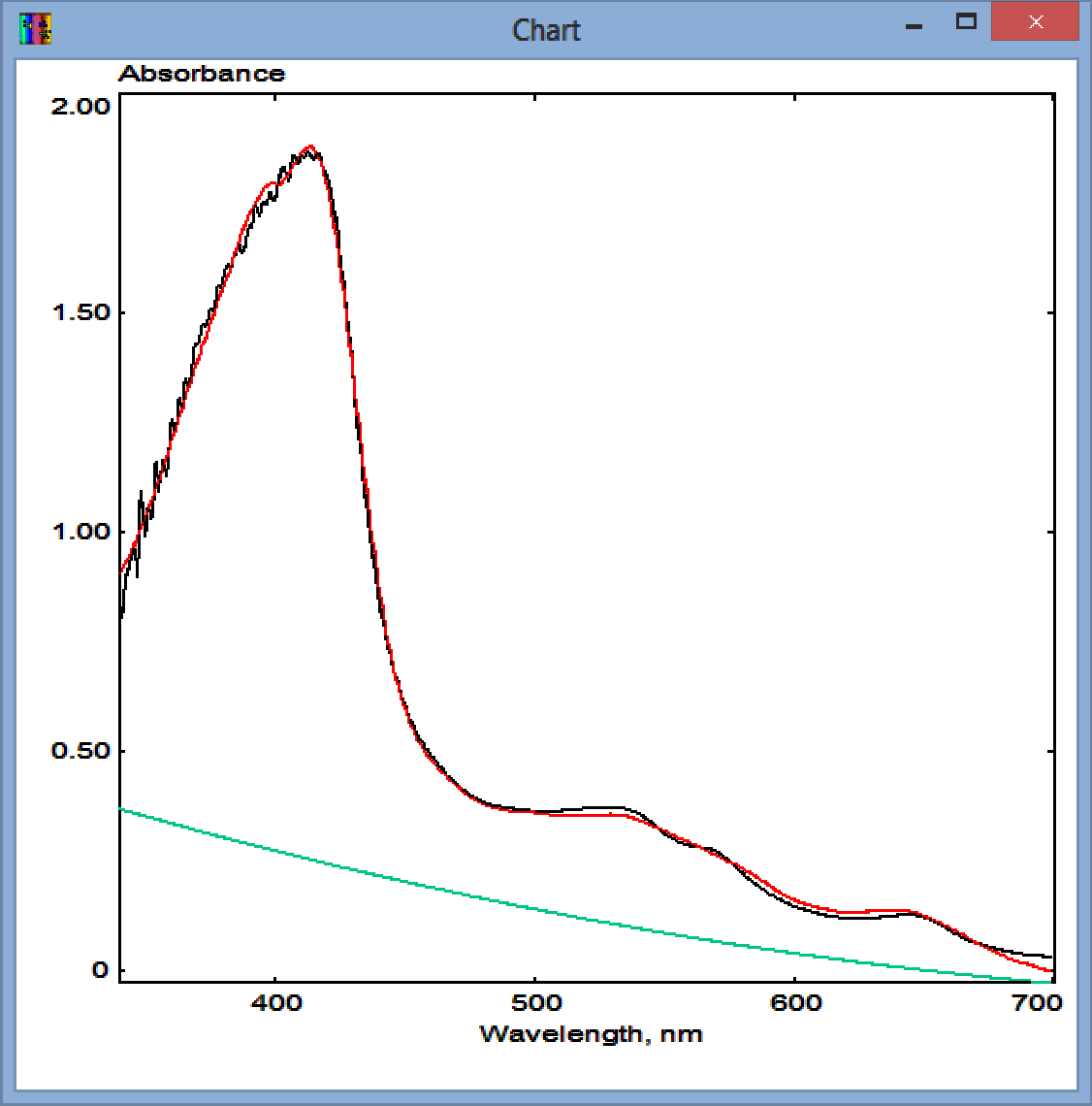
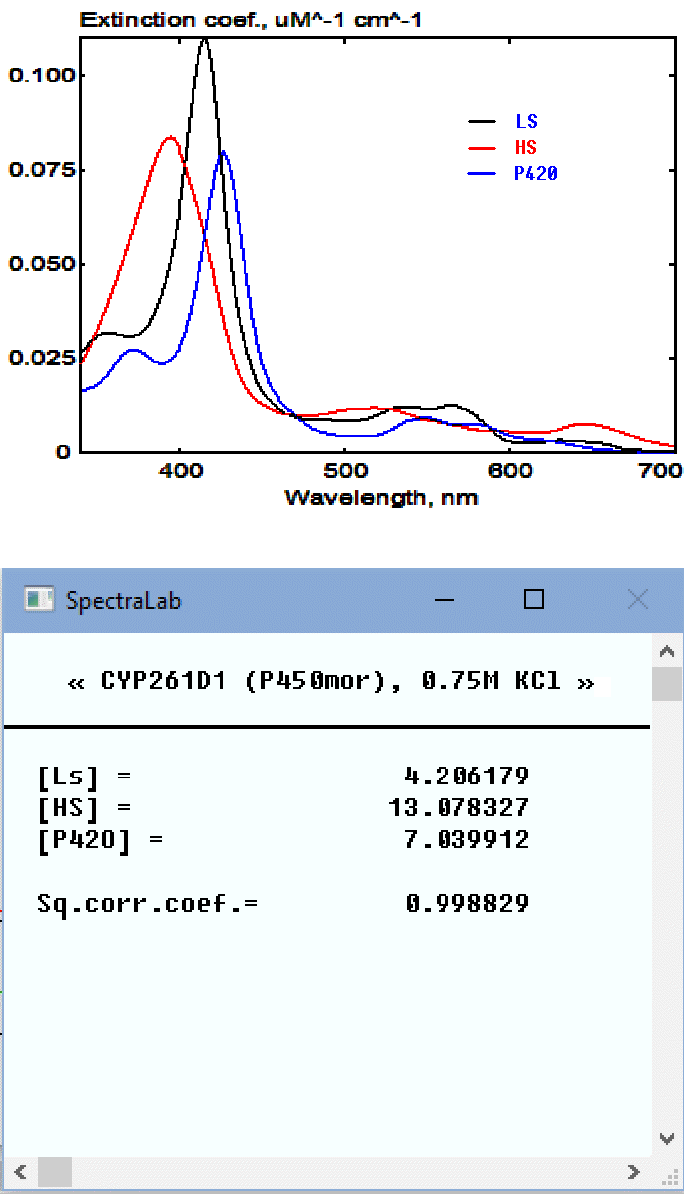
Clicking on "Run" button invokes the SURFIT procedure. Its results will be displayed in the appearing pop-up window. An example of the application of SURFIT to the analysis of the concentration high-, low- and P420 states of cytochrome P450 (purified CYP261D1 from piezophilic bacterium Moritella sp. PE36 in this case). The set of standards, which is shown in chart on the right, contained the spectra of 1 µM high-spin (HS), 1 µM low-spin (LS), and 1 µM P420 states of the heme protein. The SpectraLab Chart window and the pop-up window resulting from the application of SPAN are shown below:
        
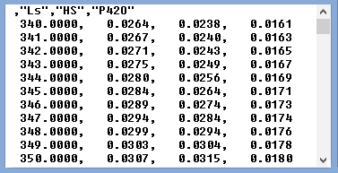
The original spectrum in the Chart pane is shown in black. The red spectrum shows its approximation with the set of standards. Its second-order polynomial part (background turbidity) is shown in green. The top line of the pop-up window contains the header of the spectrum under analysis.  The next three lines show the concentrations of the individual compounds (three different states of cytochrome P450, in this case). The square correlation coefficient for the approximation is shown in the following line. Note that all these values will also be shown in the header of the spectral trace with the results of the fitting.  As the spectral standards used for this fitting correspond to 1 µM concentrations, these concentrations are expressed in µM. The names of the compounds ("Ls", "Hs", and "P420") are taken from the first line of the file of standards. The first few lines of this file are shown below to illustrate the required format:

Basically, it is a comma-delimited file, where the first column contains the X-axis (wavelength) values, and the following columns contain the Y-values (extinction coefficients) for each of the compounds in the set. The first line contains the names of the compounds placed in double quotes and separated by commas. Note that this line should start with a comma. The wavelength range of the spectra in the file of standards should not be narrower (but may be broader) than that of the spectrum under analysis. The wavelength increment between the points should be equal to or smaller than in the analyzed spectrum. If a weighing function is needed to be associated with the standards, it should be added as a last column and entitled "Weight".