Principal Component Analysis (SPAN) module
Principal Component Analysis (PCA), a linear algebra method commonly employed to reduce the dimensionality of large datasets, is widely used for analyzing series of spectra, such as results of rapid scanning kinetic or titration experiments. It is a powerful tool that allows for resolving multiple overlapping processes and filtering out unwanted background fluctuations.
PCA analyzes a set of M individual datasets (e.g., absorbance or fluorescence) of the dimensionality N (number of data points in each spectrum). This dataset is used to construct the N × N covariance matrix, which is then transformed to find M - 1 eigenvectors paired with M eigenvalues. The combination of each eigenvector with the corresponding set of eigenvalues is termed the Principal Component. The eigenvectors may be considered unified differences between the basis spectrum and other vectors (spectra) under analysis. In a classical implementation of PCA, the basis spectrum is constructed by averaging all spectra under analysis. However, in the PCA implementation in SpectraLab, the first spectrum of the series (i.e., the spectrum taken at the reaction initiation for kinetic experiments, or the spectrum taken at no titrant added for titrations, etc.) is used as the basis.
The principal components (PCs) are sorted based on their statistical significance. The first PC represents the most typical difference between the individual datasets (spectra), and the higher-order PCs contain the less significant deviations from the basis. This way, organizing information in PC allows for reducing dimensionality without losing much information by discarding the components with low statistical significance.
In practice, each dataset may be reconstituted with increasing accuracy by successive summarizing the basis vector and the eigenvectors multiplied by the respective eigenvalues. Thus, the set of eigenvalues deduced from the analysis of a spectral series reflects the changes in the amplitude of spectral alterations represented in the respective eigenvector. Plenty of guides on PCA and its use in spectroscopy are available on the Internet. In particular, a more detailed (but yet simple) description of its principles may be found in the blog post at "Pragrammatically" wesite or a review published by Joliffe and Cadima (2016).
A distinctive, unique feature of the SPAN module in SpectraLab is the ability to combine PCA with multi-dimensional LSQ fit (SURFIT) of principal vectors with a
set of prototypical spectra (spectral standards) of the constituents of the system under study. This functionality allows interpreting observed spectral changes in terms of the concentrations of the system's constituents.
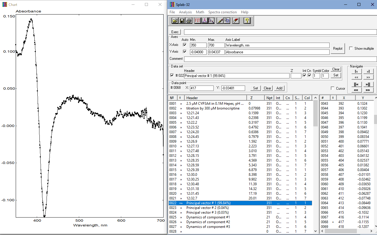
To apply PCA, the user must collect a series of spectra reflecting the changes of interest, such as reaction kinetics, protein-ligand interactions, the effect of temperature or pressure, etc. The spectra must be taken in the same spectral range and have the same number of points. The set should be placed into consecutive locations in the SpectraLab datasheet starting at the first slot. The Z-value associated with the spectra should be set at the process variable, such as time for kinetics, the concentration of the titrant for titrations, pressure for pressure dependencies, etc. The program will use the slot numbers as Z-values if the Z-column is left empty. Typically, all spectral slots below the last spectrum of the series should be empty. However, suppose the program encounters a trace with the length (number of points) different from that of the spectra found in the uppermost locations. In that case, it will be considered as not belonging to the series under analysis and deleted along with all traces located below it. The minimal number of spectra in the set is three. The maximal number is limited by the number of available slots in Spectralab. In most cases, this number shouldn't exceed 116, which leaves enough empty slots for the results of PCA in most cases. A screenshot of SpectraLab with a ready-to-analyze set of spectra before applying the SPAN procedure is shown below:
The dataset shown in the screenshot above represents a series of spectra taken in the titration of purified human cytochrome P450 3A4 by its substrate, dopamine agonist drug bromocriptine (BCT). Z-values are set to the BCT concentrations corresponding to the respective spectra. This dataset may be found in CYP3A4@BCT.SPC file in the "Examples" subfolder of the package.
To start the procedure, the user should select "Principal Component Analysis (SPAN)" in the "Analysis" section of the main menu or click on thebutton in the SpectraLab toolbar. After doing so, the SpAn parameters pop-up form appears. If the "File of standards" field in this form is left blank, the PCA procedure will be performed in its routine implementation without using its spectra fitting (SURFIT) functionality. In this case, the only parameter that affects the PCA results is "Max. number of principal components". Theoretically, the maximal possible number of PC is equal to the number of spectra under analysis minus one. However, in practice, the number of PC considered in the analysis rarely exceeds three. Clicking on the "Run" button starts the PCA procedure. The following screenshot shows the SpectraLab screen after the PCA procedure:
As seen in the screenshot above, the set of the spectra under analysis (which is not affected by the procedure) is now complemented with new traces (traces 22 - 27 in our example) with the results of PCA. The spectra of principal components ("Principal vector..." spectra, traces 22-25) are paired with the vectors of eigenvalues ("Dynamics...", traces 25 - 27). The focused spectrum, which is shown in the chart window, represents the first principal vector. In our case, it reflects 99.84% of the observed spectral changes. The respective vector of eigenvalues ("Dynamics of component #1") depicts the changes in the amplitude of this spectral transition in the process of the experiment under analysis.
It must be emphasized that the eigenvalues have no physical meaning by themselves. They must always be considered in a pair with the respective principal vector (PC spectrum). Every spectrum of the dataset under analysis may be reconstituted with certain accuracy (99.86% in terms of the sum of square deviations in this example) by adding the first principal vector multiplied by the respective eigenvalue to the first spectrum in the series. Reciprocally, multiplying the vector of eigenvalues by the Y-value corresponding to any given wavelength in the first principal vector will yield the dependence of optical density at this wavelength on the Z-value (substrate concentration, in our example).
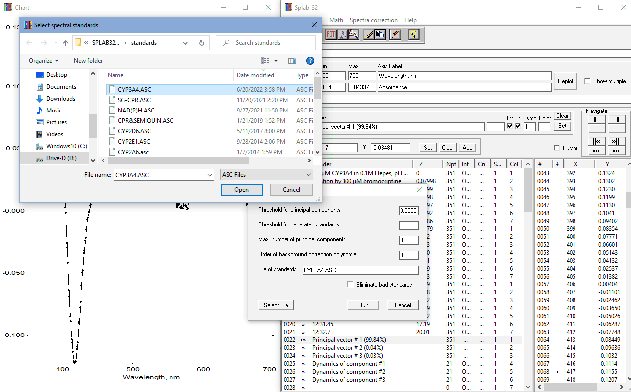
If the prototypical absorbance spectra of the individual components of the system are known, the results of PCA may be interpreted in terms of the changes in concentrations of the system's constituents. To use this option, the user should provide a file containing prototypical spectra of known concentrations of the compounds under study. The format of these ".ASC" files is described in the SURFIT section of this help. By default, these files should be placed in the "Standards" subfolder of the package. The names of the compounds should be specified in the first raw of the file. If a weighting function needs to be used, the column with the weighting table should have the word "Weight" as its header. In case the system contains a chromophore that, although absorbing in the monitored spectral region, is not involved in the transitions under study (i.e., a compound that remains at a constant concentration in the experiment), its name should be marked with an asterisk symbol (*).
In the example shown in the screenshots above, to analyze the substrate-induced changes in cytochrome P450 3A4 (CYP3A4), we have to consider the transitions between three forms of the enzyme - so-called low-spin, high-spin, and P420 states, which differ in their spectral properties. The binding of BCT is known to displace the equilibrium between these states towards the high-spin form. Spectral standards of these three states are available in the file CYP3A4.ASC in the "Standards" subfolder of the package.
To repeat the PCA procedure with the same dataset using CYP3A4 spectral standards, one does not need to delete the traces resulting from the previous PCA round - they will be automatically deleted and replaced with the new results. After clicking on the "Select file" button in the Span parameters form, the user will be given an option to select the file with spectral standards located in the "Standards" subfolder of the package:
Other parameters in the SpAn parameters form related to the use of spectral standards in PCA are:
After reviewing and adjusting these parameters, the user may click on the "Run" button. The protocol of PCA that appears in the new window at the end of the analysis contains information about the results of approximation of the principal components by spectral standards and the parameters used in calculating the changes in the concentrations of the species under analysis. An example of this protocol is exemplified on a separate page.
- Threshold for principal components - a threshold of the square correlation coefficient (R2) used to consider principal components significant. The program will attempt to approximate all principal components by a combination of given standards. The components with R2 below the given threshold will be discarded from consideration.
- Threshold for generated standards - The program will attempt to approximate the given standards by a combination of spectra in the dataset under analysis. If this approximation yields the R2 value above the given threshold, the new "generated" standards will be used in calculating the concentrations instead of the originals. The original standards will always be used if this threshold is set to 1. This feature is used when the spectral properties reflected in the used standards may differ from the actual properties of the compounds under study (e.g., if the standards were obtained with a different isoform of the protein).
- Max. number of principal components - the number of principal components to be considered. All higher-order components will not be shown. The maximal possible number of PC is equal to the number of spectra under analysis minus one.
- Order of background correction polynomial - The order of the polynomial component for the fitting of the principal vectors by spectral standards. It may vary from 0 to 3. It is recommended that, prior to the final round of PCA, the user probes the optimal order of the polynomial component by fitting (with SurFit procedure) the base spectrum (the first spectrum of the series) and the Principal Vectors with the chosen set of standards and varying polynomial order.
- Eliminate bad standards - This checkbox may affect the fitting results only if a value below 1 is specified as the "Threshold for generated standards". In this case, if this checkbox is checked, the concentration of all compounds whose generated standards yielded the R2 value below the threshold will be considered constant (not changing in the experiment under analysis).
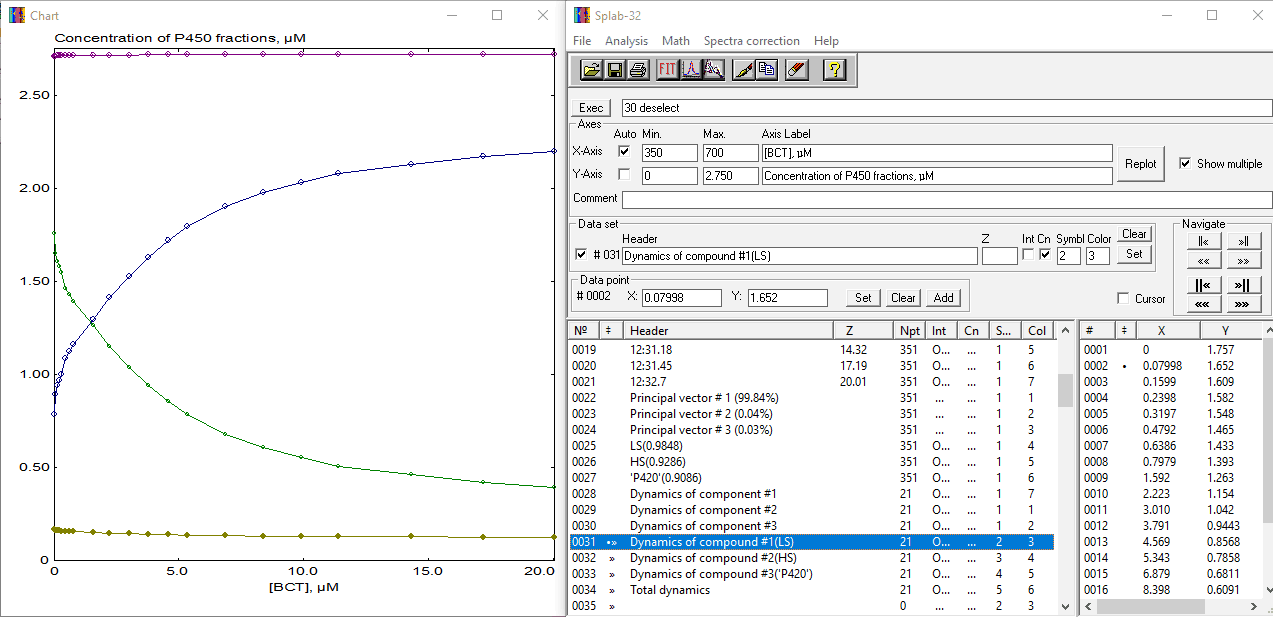
The screenshot of the SpectraLab screen with the results of applying the PCA with the spectral standards is shown below:
As seen from this screenshot, the traces with Principal vectors and Eigenvalues ("Dynamics of component") are now complemented with a set of newly generated spectral standards and a set of traces reflecting the changes in the concentrations of the compounds under analysis (traces 31 - 34). These four traces are shown in the Chart window, where LS is in green, HS - in blue, P420 - in dark yellow, and the total of all three P450 states is shown in magenta. Now we can divide trace 32 by trace 34 to obtain a dependence of the fractional content of the high-spin state on BCT concentration and fit it to the "tight binding" equation ("Ligand binding" model, submodel 1 in CURFIT module). Note that prior to fitting, we have to set the Z-value associated with this trace to the total concentration of CYP3A4 protein in our sample - this value may be taken from the arithmetic mean of trace 34 (it is equal to 2.72). Here is the final result of our analysis: