Non-linear least square (NLSQ) fitting is one of the most common tasks in data analysis. Although several commercial software is available, SpectraLab provides its own curve-fitting tool (CURFIT). It allows the user to fit the results of spectral analysis to equations commonly used in (bio)chemical research in situ, without transferring data to another software.  CURFIT provides better flexibility and tune-up options than most commercial NLSQ software. It combines two different methods of optimization - Nelder-Mead and Marquardt techniques. While the Marquardt algorithm usually provides more rapid convergence in the proximity of the minimum, the Nelder-Mead (simplex) technique is less local and provides better convergence when the initial estimates are far from the optimum.

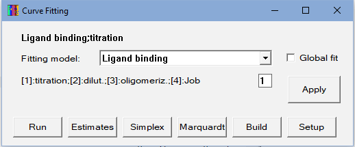
To perform the CURFIT procedure, the user should place the line-cursor at the trace to be fitted (or one of the traces selected for global fit) and select "Curve fitting (CURFIT), Non-Linear Regression" in the "Analysis" section of the Main Menu. CURFIT may also be invoked by clicking at   button in the SpectraLab toolbar. Upon invoking the CURFIT, the following form appears:

The top line shows the name of the currently selected fitting model. To change the selection, one should click the down-arrow button next to the "Fitting model" field. Then, a drop-down list of predefined models will be accessible for selection:

  

A complete list of the available models and a description of the underlying mathematical equations may be found in the "Mathematical models implemented in CURFIT" section of this Help. For some of the models, the user should make a selection between several variants or specify the value of an additional parameter:

The checkbox "Global fit" allows the user to perform a global fit of multiple selected traces. If selected, the fitting procedure will be applied to the whole set of selected traces (marked with the "»" symbol in the list of traces).

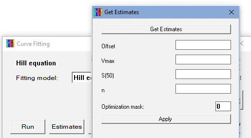
Clicking on the "Run" button initiates the fitting procedure. It starts with invoking the user to specify the initial estimates of the parameters under optimization. Clicking on the "Get estimates" button in the appeared form causes the program to suggest possible estimates on its own:

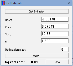
The user can specify the initial estimates if they are known or alter the suggested values. Upon clicking on the "Apply" button, the program calculates the fitting curve, displays it in the "Chart" window, and shows the respective square correlation coefficient in the "Get estimates" window (see illustration on the right). The "Optimization mask" parameter allows the user to exclude certain  parameters from optimization. This is a "bit-mask" - each parameter has its corresponding "power of two" values - 1, 4, 8, and 16 for the Offset, Vmax, S(50), and n (the Hill coefficient) in the Hill equation case shown above. Setting the mask to 1 means that the Offset will be fixed at its initial value. Setting the mask at 16 will cause fixing the Hill coefficient (n). If the mask is set to 17, both the Offset and and the Hill coefficient will not be changed in optimization (17=16+1). In most cases, the mask should be set to 0 to allow the optimization of all parameters of the model.

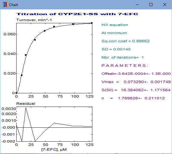
 Clicking on the "Done" button starts the optimization procedure. For most models, the Simplex (Nelder-Mead) and Marquardt algorithms are applied successively. The progress of the fitting will be displayed in the pop-up window. Optimization may be interrupted at any time by pressing the "Esc" key on the keyboard. When at least one of the criteria selected for the end of optimization (see below) is reached, the process stops, and the results of optimization are displayed in the "Chart" window:

The top graph in this output shows the dataset under fitting along with the fitting curve. The graph at the bottom shows the plot of residuals. The reason for stopping the optimization is shown under the name of the model on the right side of the chart. These reasons may be as follows:

• At minimum - the optimization is at minimum. Any attempts to improve the fitting further has failed (this is the best possible case!)
  
• Changes are less than ...%  - the changes in all parameters in the last iteration were below the limit specified in the "Setup" form
  
• Sq.corr.coef. is higher than ... - The square correlation coefficient reached the threshold specified in the "Setup" form.
  
• ... iterations performed - the last applied optimization method performed the maximal allowable number of iterations specified in the "Setup" form.

Besides these "good" or "rather good" reasons above, there are three reasons indicating that the fitting has failed (or interrupted):

• !!! Interrupted by user !!! - the user pressed the "Esc" key during optimization
  
• !!! Matrix invert error !!!  - matrix inversion error in Marquardt optimization
  
• !!! Matrix is singular !!! - matrix singularity in Marquardt optimization.
  

The latter two messages usually indicate that the optimizing parameters reached the values, where the mathematical model is ill-defined. The user may attempt to repeat fitting with another set of initial estimates. The fitting results chart may be re-invoked at any time by placing the cursor-line on any already fitted trace and clicking on the button in the toolbar. 

While clicking on the "Run" button initiates the entire sequence of steps of fitting, the buttons "Estimates", "Simplex", and "Marquardt" provide an option to invoke these steps separately at user's discretion. 

The criteria for stopping optimization along with the optimization fine-tune parameters may be adjusted in "Setup" :

This form is accessible upon clicking on the "Setup" button in the main "Curve fitting" form. Note that the "Setup"  window appears below the "Chart" window. So, to have it accessible, the user should decrease the height of the Chart window to leave some space below it. This inconvenience might be considered a bug. It will be fixed in further releases. The top three lines of this form contain the criteria for stopping the optimization procedure. Relative accuracy defines the minimal fractional change of optimizing parameters per iteration. For instance, the value of 1E-5 requires the program to stop optimization when the changes of all parameters are less than 0.001% of their values per iteration. The next two lines contain the fine-tune parameters of the Marquardt algorithm - the dumping factor (λ) and the dumping increase/decrease factor (ν). For a description of the effect of these parameters on optimization, the user may refer to Marquardt 1963 or the description of the algorithm by H.P. Galvin. However, specifying these parameters is optional. If the "Marquardt auto-set" checkbox is checked, the program sets the optimal λ and ν automatically and ignores the values entered in the Setup form. The "Simplex size" parameter defines the initial size of simplex in the Nelder-Mead algorithm. It is expressed as a fraction of the initial estimates of the parameters under optimization. A larger simplex size makes the procedure less local and increases the chances of reaching the global minimum, even if it lies far from the initial estimates. After pressing the "Apply" button, the parameters are set and saved. They will be re-loaded at the next start of the SpectraLab (i.e., they are preserved between the sessions). 
   
In addition to performing curve fitting, one can also use the "Curve fitting" form to build a theoretical curve for the selected fitting model and a given set of parameters. To do so, one should place the cursor-line at an empty slot of the curve list and invoke CURFIT through Main Menu or the toolbar.  If the desired model uses the trace-associated Z-value, it must be entered beforehand. After selecting the model and pressing the "Build" button in the "Curfit" form, the user should specify the desired parameters in the appeared pop-up window. After clicking on the "Done" button, the user will be asked for the minimal and maximal values at the X-axis and the number of points in the trace to build (the points will be evenly distributed).   The default values for the X-axis limits are taken from the X-axis "Min." and "Max." fields in the top pane of the SpectraLab main window.